Sonja Schneider did her honours’ project at the International Center for Numerical Methods in Engineering (Barcelona)
and was supervised by Dr. Roland Wüchner (TU Munich), Ing. Jordi Cotela (CIMNE) and Dr. Riccardo Rossi (CIMNE).
Introduction
The Honours Project deals with the implementation of an overlapping chimera method based on a Dirichlet-/Neumann coupling for convection-diffusion problems. The focus lies on the implementation of two different solution methods for using the chimera technique.
The iterative solution method is based on a convergence of the solution with the help of iterations. In each iteration, the interface values (Dirichlet- or Neumann transmission conditions) of the corresponding domains are updated and the domains are solved independently. One big disadvantage of this method is, that there is the possibility that the solution does not converge.
The second solution method is a monolithic one. The basic idea of the monolithic method consists in the creation of one big equation system which contains the equations of both domains. The coupling between the domains is implicitly integrated in this equation system. The big advantage of this method is, that the solution is obtained in one iteration step. However, this method can become computationally very expensive when a lot degrees of freedom are involved, which leads to a huge equation system.
What is the Chimera Method?
The idea of using a Chimera method is to apply a fine body-fitted mesh around an object and to apply a coarse background mesh in the rest of the domain. This means that one gets a high resolution of the region of interest around the object and a lower resolution farer away from the object by the background mesh. In this way, one can save computational costs.
Furthermore, the background mesh does not have to fill out the whole considered domain. In the region where both meshes are overlapping, the background mesh can be erased or neglected in the solution process after a certain overlapping distance.
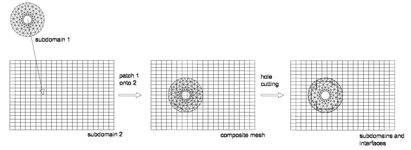
The solution procedure of the Chimera method consists of two steps: the hole cutting in the background mesh and the coupling of the sub-domains (see Fig.1).
In the hole cutting process, it has to be figured out which elements of the background domain located inside the patch mesh can be neglected in the solution procedure. These hole elements can be taken off in the background mesh to create the interfaces of the sub-domains. This step is needed to enable the establishment of the coupling. The resulting background mesh consists therefore of the original elements without the hole elements and the interface consists in the element faces bounding to the hole. This newly created interface is needed in the coupling step to couple the background- with the patch mesh.
 |
|
Fig.1: Steps of the Chimera Method (taken from [1])
|
The Coupling Conditions
The coupling conditions on the interfaces of the sub-domains have to be chosen in that way such that a continuous solution over the whole computational domain can be achieved. The Chimera method in this project is based on a Dirichlet-/Neumann coupling. The underlying model equation of this project is the convection-diffusion equation.
Therefore, the Dirichlet-coupling consists of the exchange of temperature values between the sub-domains whereas the Neumann-coupling consists of the calculation of flux values on the corresponding interface nodes:
with υ being the viscosity, q the flux calculated by velocity gradients and n the normal vector on the interface.
The flux term is hereby naturally introduced if one partially integrates the diffusion term by using the weak form of the convection-diffusion equation.
The Iterative- and the Monolithic Method
In this section both solution methods are shortly introduced.
The Iterative Method
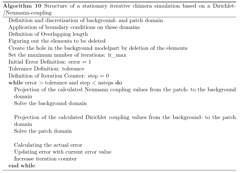
As told already, the iterative solution method is based on a convergence of the solution with the help of iterations. In each iteration, the interface values (Dirichlet- or Neumann transmission conditions) of the corresponding domains are updated and the domains are solved independently. One big disadvantage of this method is, that there is the possibility that the solution does not converge. In Fig.2 the workflow for a stationary solution process is presented. It is assumed that the Dirichlet coupling takes place on the interface nodes of the patch domain and the Neumann coupling takes place on the fringe nodes of the background domain.
 |
|
Fig.2: Steps of an iterative chimera simulation
|
The Monolithic Method
The basic ingredient of this method is, that the equation system of each domain is combined into one big global equation system. The coupling conditions of the Dirichlet-/Neumann coupling are then implicitly applied by modifiying this global system.
The big advantage by using this direct coupling is, that the equation system can be directly solved in one iteration step. A drawback for an equation system with a huge amount of degrees of freedom is, that it can be computationally expensive to solve it by a direct solver.
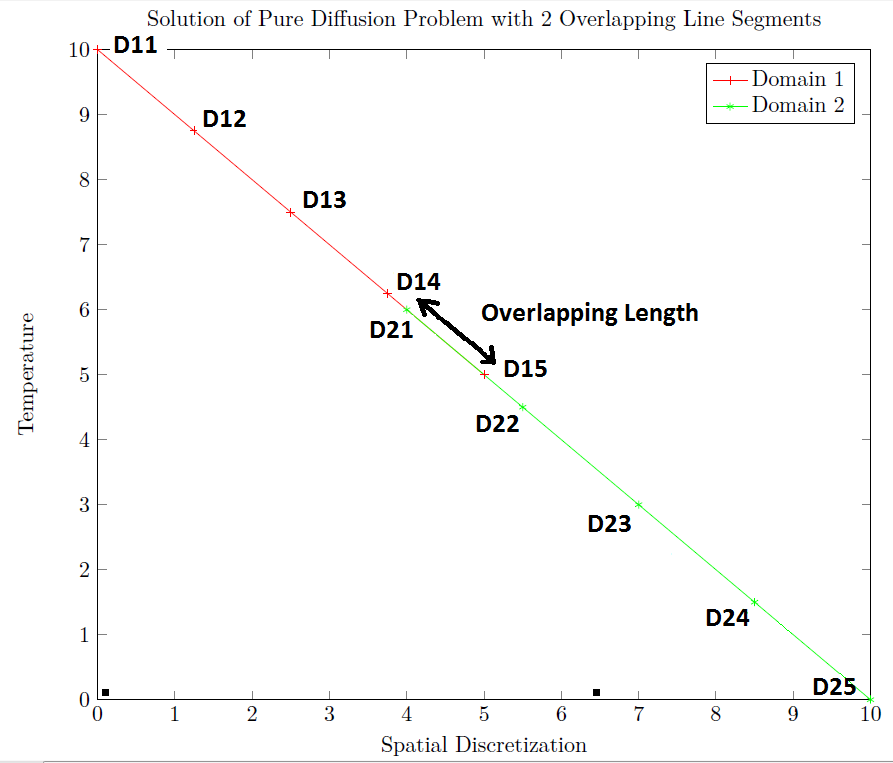
In the following, the basic scheme and theory of the direct coupling are illustrated. This is done based on a one-dimensional example of two-overlapping line segments (see Fig.3). The underlying model equation is the convection-diffusion equation.
 |
|
Fig.3: Steps of a monolithic chimera simulation
|
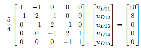
The starting point for the creation of the monolithic solution are the global equation systems for Ω1 and Ω2 :
 |
 |
|
(a) Global equation system for Ω1
|
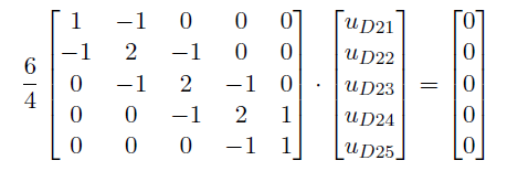
(b) Global equation system for Ω2
|
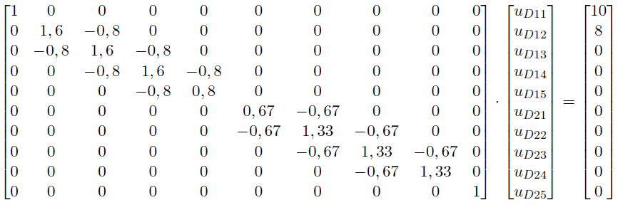
The next step in the solution process consists in establishing one global equation system for both domains according:
 |
|
Fig.5: Unified Global Equation System
|
The value for the Dirichlet coupling is coming from line segement 2. Therefore, the corresponding row (row of uD15) of the stiffness matrix is set to zero and the diagonal value is set to one. Then, it is searched for the nodes of the host element in which the boundary node falls. These nodes are taken into account in the interpolation process. On the corresponding column of the degrees of freedom of these interpolation nodes (uD21 and uD22) the negative values of their shape functions (denoted in the matrix as -NDoF) are positioned in the row of the boundary node (uD15). The sum of the shape function values sum up to one. For instance, the shape function value NuD21 is the value of the shape function of node D21 evaluated at node D15.
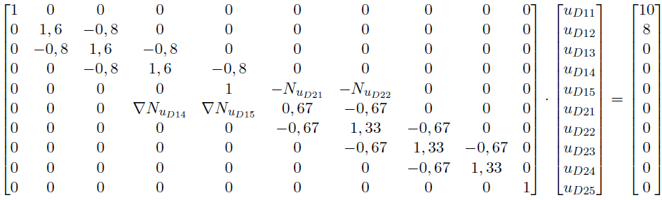
The transmission condition at the left end of line segment 2 is a Neumann condition. The only difference to the application of the Dirichlet condition consists in the application of the shape function derivatives (denoted in the matrix as ∇NDoF) multiplied with the normals (flux value) instead of only the values of the shape functions. If one sums up these values, the result has to be zero. Furthermore it is not necessary to set the corresponding row to zero and its diagonal to one. The equation system is therefore transformed like that:
 |
|
Fig.6: Final Global Equation System
|
The Test Cases
After the implementation of both solution methods, studies were performed on two test cases to explore the strength and weakness of each solution method. The main focus lies hereby in two main aspects. When coupling two overlapping meshes, an important question is how long the overlapping distance of the two sub-domains has to be. Thereby, it is interesting to investigate the minimal overlapping distance needed so that the method works. Further, it is interesting to see the simulation time needed depending on the used overlapping distance.
In the following, the test cases are shortly presented.
Test Case 1
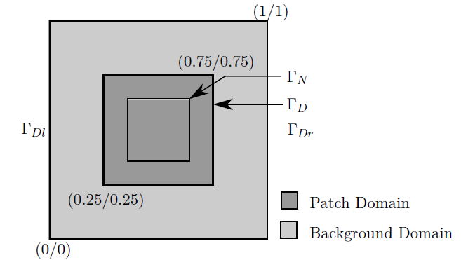
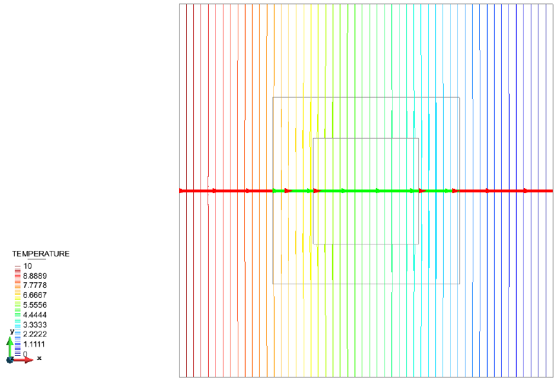
The setup of the test problem is shown in Fig.7. The left wall of the background domain (ΓDl) is fixed to 10°C. The right wall of the background domain is fixed to 0°C. On the background fringe nodes the Neumann transmission condition is applied to get a well-posed problem whereas a Dirichlet condition is applied on the interface of the patch domain.
 |
 |
|
(a) Geometry of test problem 1
|
(b) Solution of test problem 1
|
Test Case 2
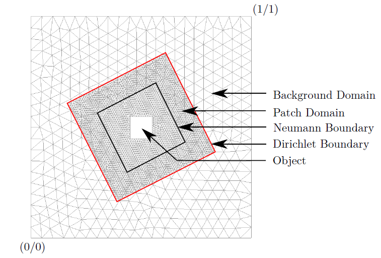
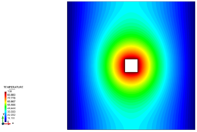
The problem definition is illustrated in Fig.8. The patch mesh is spanned up by the two points P1 = (0.25/0.25) and P2 = (0.75/0.75). It is rotated by 27° around its center. The left- and the right wall of the background domain are fixed to 0° whereas the object is fixed to 100°.
 |
 |
|
(a) Geometry of test problem 2
|
(b) Solution of test problem 2
|
Conclusions
After the implementation of both solution methods, two test cases were presented to compare both methods.
Generally it was found out, that if the convergence criteria of the iterative method is kept strict, then both solution methods deliver the same solution quality. By increasing the mesh size, the simulation time decreases exponentially in both solution methods.
One elaborated feature of the monolithic solution method is, that simulations can be conducted with much smaller overlapping length where the usage of the iterative method is not anymore possible.
A further feature of the monolithic method is, that the simulation time nearly stays constant if one varies the overlapping length compared to the iterative method where the simulation time increases drastically.