Optimization Algorithms for Full Waveform Inversion

Viola Muning Li

The Honours Project was completed at the Chair of Computational Modeling and Simulation and was supervised by Tim Bürchner, M.Sc.

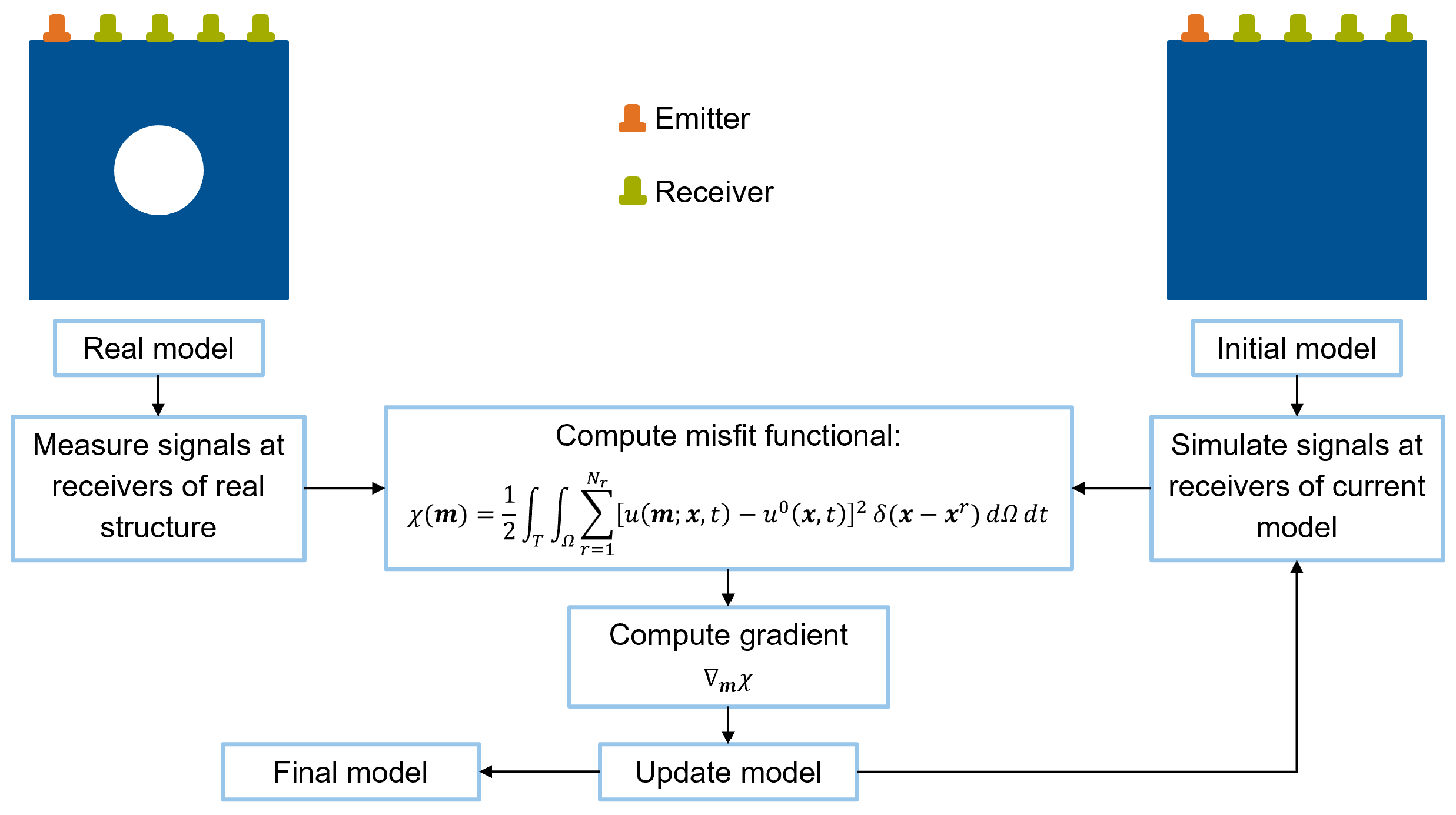
The Full Waveform Inversion (FWI) is an imaging technique based on ultrasonic wave propagation. Originating from
seismic tomography, it is also a
useful tool for the non-destructive testing of structures. Using the FWI it is possible to gain insight into the
inner structure of a medium and to detect the position and
shape of voids. The main idea is to excite the medium with ultrasonic pulses and to
measure the resulting waveforms at different
receivers. These waveforms will be different than the waveforms obtained by solving the wave equation for a
homogeneous medium without any defects. By minimizing this
misfit between measured and computed waveforms it is possible to reconstruct the real structure.

The minimization of the misfit poses an optimization problem that is typically solved using non-linear
gradient-based iterative optimization methods.
The gradient with respect to the model parameters can be computed efficiently with the adjoint method. A
detailed discussion of the FWI and the adjoint method can be
found in [1]. Figure 1 shows the general workflow of the FWI.

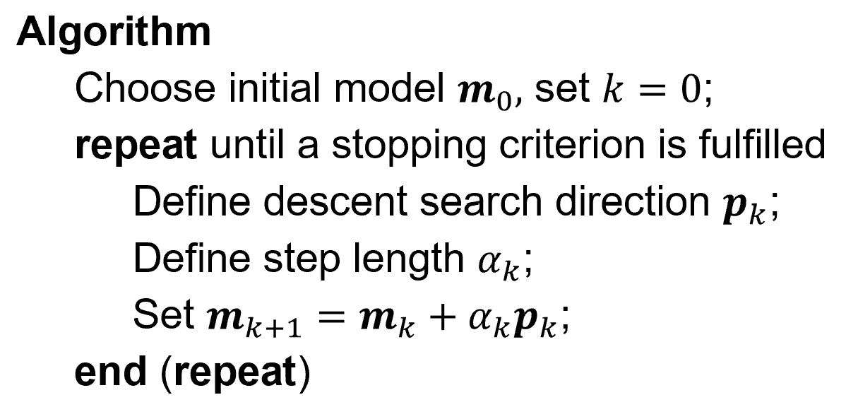
In the following, all optimization methods, if not stated otherwise, follow the discussion of Nocedal and
Wright [2]. Figure 2
shows the pseudo-code of a general iterative optimization method.
Starting from an initial model, a descent search direction is defined along which an appropriate step length
has to be chosen. A very common choice is to select a
step length that satisfies the Wolfe conditions. The Wolfe conditions make sure that in every iteration a
reasonable progress is made by looking at the value and curvature
of the objective function.

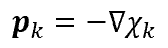
Two of the most simple iterative optimization methods are the steepest descent method and the non-linear
conjugate gradient
method. The steepest descent method selects,
as the name suggests, the steepest descent direction as the search direction. Thus, the search direction is
simply
the opposite of the gradient:

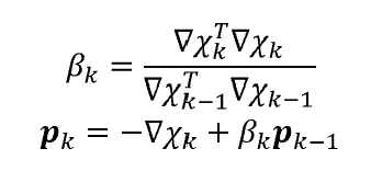
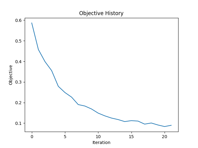
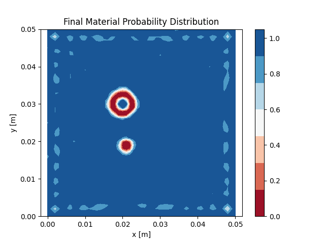
The non-linear conjugate gradient method is a generalization of the linear conjugate gradient method, where all
search directions satisfy the conjugacy condition.
In the first iteration, the search direction is chosen to be the steepest descent direction. The subsequent
search directions are updated using for example
the Fletcher-Reeves update rule:

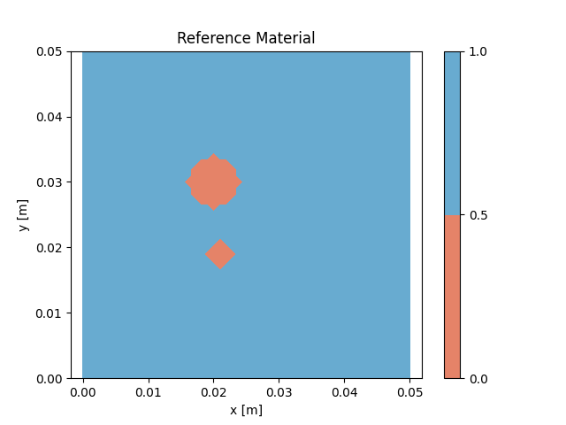
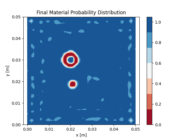
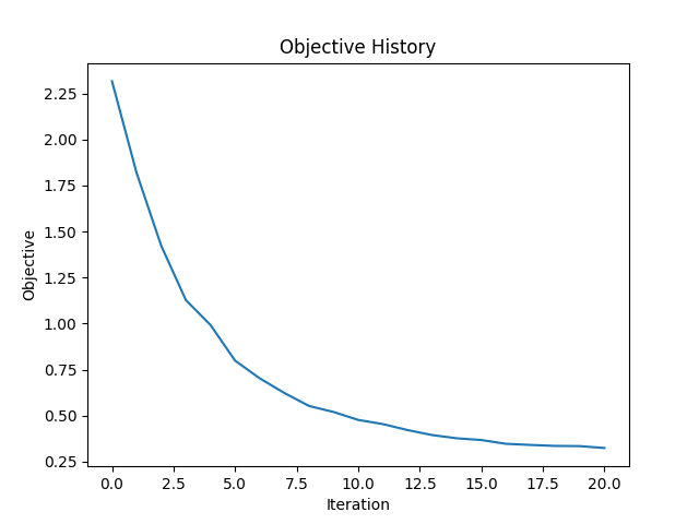
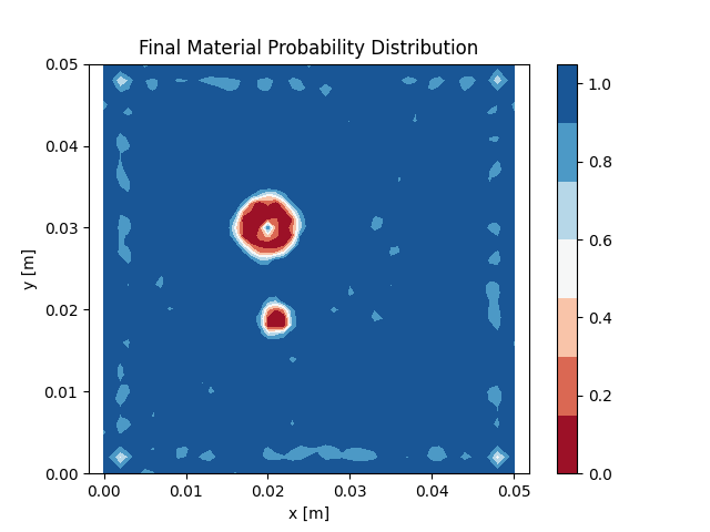
The two methods described above are applied to a medium with two circular voids and otherwise homogeneous
material distribution. Figure 3 shows the
reference model. In total 20 emitters and 20 receivers
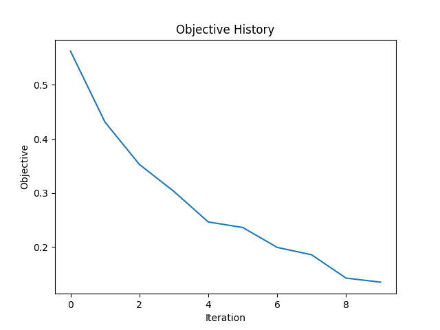
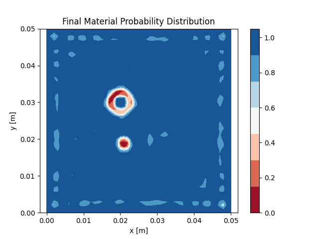
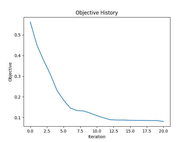
are placed all around the structure. This means that 20 simulations are conducted in each iteration. Figures 4
and 5
show the objective history over the iterations and the
final
material distribution of the optimized model. Both methods
are able to capture the main features of the two voids, but can not reproduce them perfectly.

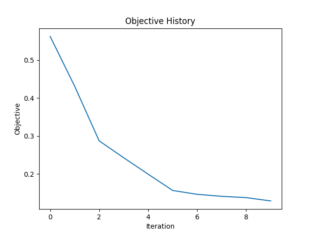
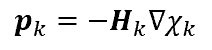
The steepest descent method and the non-linear conjugate gradient method only use first order information,
namely the gradient, which in general can lead to a slow
convergence. More advanced methods such as Newton’s method use also second order information. Here, the
search direction is updated using the Hessian of the objective
function. This leads to a very good convergence rate, but the second derivative is often very costly, especially
for
high-dimensional problems. The limited-memory BFGS
method solves this issue by finding an approximation to the inverse Hessian which is then used for the search
direction:

This method is called limited-memory BFGS because instead of storing the typically dense matrix, only a
small number of vector pairs is stored:

These vectors are then used to construct the approximation matrix.

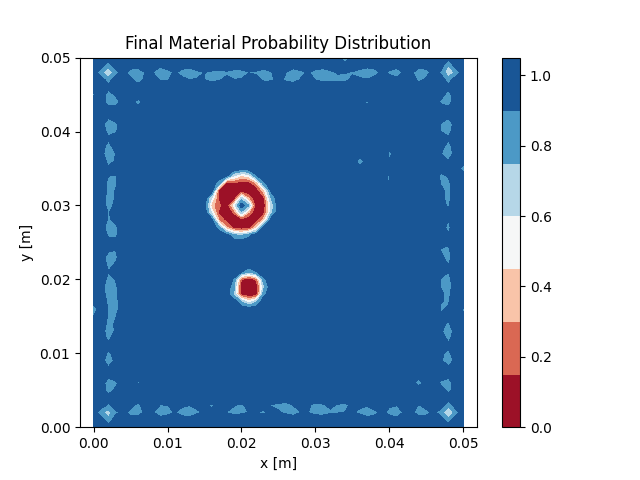
Figure 6 shows the results of the problem using the L-BFGS method. One can see that a smaller objective
function value is obtained and that the final material
distribution is also slightly better. Another advantage of the L-BFGS method is that it can be extended to
solve
constrained optimization problems with bounds defined on the optimization
variables, as presented in [3].

This rather simple example with 2601 degrees of freedom, 4000 time steps, and 20 emitters took 5690 seconds for
the complete optimization process. This can quickly become infeasible when considering
more complex examples. Fichtner [1] therefore proposed a data reduction technique called source stacking.
Instead of solving the wave equation separately for each emitter, several emitters
are triggered simultaneously. The cost of this is equal to the cost of a simulation with one emitter only. The
receiver signals are then the sum of all signals due to each individual source. This
leads to the drawback that the receiver signals can not be separated afterward and some information is lost
due to the superposition of waves. In general, a better result can be expected
when fewer sources are stacked together. Figure 7 shows the same example as before, but this time 4 emitters are
triggered
simultaneously. This means only 5 simulations are necessary instead of 20
in each iteration. The prediction quality is comparable to the one obtained using the L-BFGS method, but the
computation
time decreased from 5690 seconds to 1408 seconds.

Another method, which can reduce the numerical cost significantly, is called multi-batch L-BFGS and was
presented in [4],
[5]. In the standard mini-batch approach, the data, or in this case the different experiments, are divided into
smaller batches. In each optimization interation, the model is then updated with respect to one batch only. The
problem with using L-BFGS with the standard mini-batch update scheme is that
the updates can become unstable when gradients are based on different experiments. The solution is to have an
overlap between two consecutive batches and to base the update only on those experiments
which overlap:

The result of using this method is shown in Figure 8. Again the prediction quality is comparable to the one
obtained using the L-BFGS method while the computation
time decreased to 2886 seconds.

References