Predicting Thermal Fields using Surrogate Models for Laser Powder Bed Fusion of Metals

Jalal Helou

This honours project was performed at the Chair of Computational Modeling and Simulation (TUM)
and
was supervised by PD Dr.-Ing. habil. Stefan Kollmannsberger and Vijaya Holla, M.Sc.

Motivation

Laser powder bed fusion is an additive manufacturing technology that utilizes the melting
properties of metals to build intricate three-dimensional metal parts that are not feasible by standard metal processes.
This is done by focusing a laser onto the powder bed, at which the particles melt and solidify. Common metals used in this
process are Aluminum, Steel, Stainless Steel, and Copper [1]. Several methods of laser powder bed fusion exist, such as
Selective Laser Melting (SLM) and Selective Laser Sintering (SLS).

Numerical simulations of laser powder bed fusion present several challenges due to the small scale
of the melt pool at each laser location. Additionally, for any real use case, simulating the manufacturing of a
part will require a numerous number of layers and a kilometers of distance to be covered by the laser path.
As for the time scale, small time steps are required in order to accurately represent the merging of the melt pools
along the laser path [2]. Thus, full scale simulations require large computational cost and are not currently feasible
for complex parts.

This work is part of an effort to develop a surrogate model for transient heat simulations for laser powder bed
fusion, specifically Selective Laser Melting (SLM). A machine learning model is trained for the estimation of steady
state heat evolution around the laser. This model would later be used as part of a multi-scale model that would utilize
the surrogate model for the local laser temperature field, while a coarse FEM simulation solvers for the far field temperature
evolution. This approach is expected to decrease the computational cost accompanied with SLM simulations, while maintaining an
acceptable level of accuracy.

Pre-processing

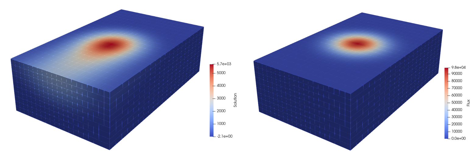
The data available was generated from 88 different simulations, performed at different laser velocities and powers, with ranges of 200 to 750 mm/s
and 50 to 450 Watts respectively. Each simulation included a flux field applied by the laser and the temperature field resulting from solving the
convection-difussion equation over a finely meshed 1000 x 600 x 300 µm domain. An example can be seen in Figure 2.

In preparation of the available data, the following operations were performed:

• Computation of the temperature gradient field
• Using half of the field, in order to exploit the symmetry of the problem
• Computation of the distance to the laser center for every point available, later used as an input to the neural network
• Loading the data into PyTorch using Paraview’s Python API

Afterwards, there were 676,200 points per simulation, with the following known quantities:

• Three-dimensional coordinates, with the origin attached to the field’s corner
• Distance to the laser center
• Flux of the laser
• Velocity of the laser
• Power of the laser, in Watts
• Resulting temperature

All the mentioned parameters are normalized using the AbsMaxScaler from sklearn’s Python library. The scaler ensures that the maximum absolute of each parameter is 1, wihtout shifting the center of the data.

Sampling

With the large number of data points available, along with the high variation of the temperature
across the field, the sampling method would have a large impact on the quality of the prediction. Thus,
several methods have been experimented with. Alongside a random distribution, the following methods were
studied:

Laser-Based Sampling:

This method utilizes the distance to the laser center of each point in the field, and samples points with a
probability that is inversely proportional to this distance, as seen in Figure 3. As a result, the neural network would obtain data points
that are in the close vicinity of the laser.
When used, this distribution has caused the neural network to overestimate the temperature values in the points away from the
laser center.

Gradient-Based Sampling:

This method utilizes the magnitude of the gradient of the temperature field, with the sampling probability
being proportional to the gradient, as seen in Figure 3. As a result, the neural network would train with points that are at the
large shifts in temperature.
Using this method, the neural network was able to better capture the changes in temperature throughout the
field, while slightly overestimating the low temperatures at data points away from the center.

Following experimentations with these methods, the best generalization result was obtained with a mixture of
random sampling and gradient-based sampling.

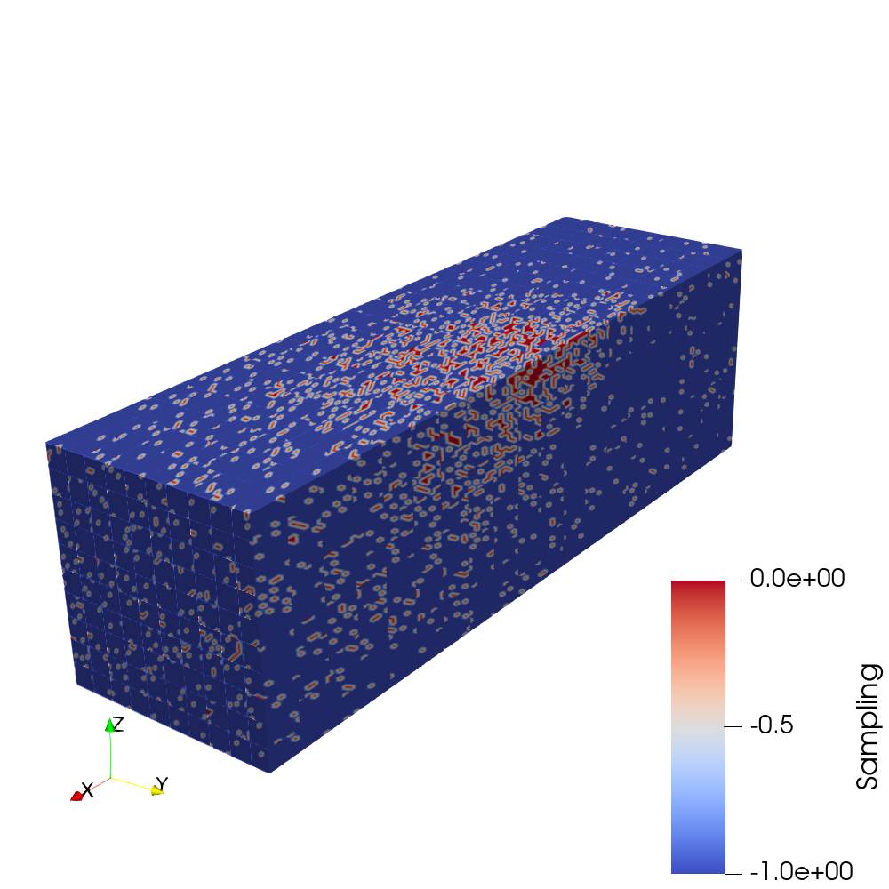
As for the number of sampled points and files, they were limited by the available computational memory at the CIP Pool machine of the project.
The Nvidia™ Quadro P2000 at the project’s machine could not be used due to its limited memory of 2 GB, preventing any GPU-accelerated training.
Therefore, the 32 GB of Random-Access Memory available dictated the amount of sampled points and the number of files to be used in the training, which was performed on the Intel™ Core i7-7700K CPU. Finally, 7 % of the data points were sampled per file, from 35 files sampled randomly from the 88 files. An example of this sampling is shown in Figure 4.

Neural Network Architecture

Over 40 different neural networks were trained with different combination and dimensions of the following layers from the PyTorch library:

• Linear + ReLU
• Linear + LeakyReLU
• Linear + LeakyReLU + BatchNorm
• Linear + PReLU
• Linear + PReLU + BatchNorm
• Linear + Sigmoid
• Linear + Sigmoid + BatchNorm

The deepest networks comprised of 12 hidden layers of dimension 100 each.
Each neural network was trained for 2-3 days on the TUM BGCE Computer Lab
machines utilizing the CPU due to the large number of points.

Python Workflow

Due to the time needed for training the networks and the repetitive nature of the operations, a Python workflow was developed. The focus of the
code was to be as modular as possible, as the direction of the project was to experiment and evaluate different methods for the surrogate model,
whether during the project or for further developments.

The workflow was split into the following parts:

Pre-processing

1. Sample N simulation result files
2. Read fields using Paraview’s Python API
3. Sample using the user-defined sampling weights for the different sampling methods (random, laser-based, gradient-based)
4. Scale using AbsMaxScaler()

Training Loops

Looping over the user-defined combinations of dimensions and layer types, the following is performed for each architecture:

1. Start training loop up to N user-defined epochs
2. Calculate the change in Mean Square Error cost over the last 1000 epochs:
   • If the change is less than 1%, half the learning rate and restart the training.
   • If the change is increasing and the training starts to diverge, decrease the learning rate by 1/3 of the current, and restart the training.

Post-processing

1. Evaluate neural network over non-training files
2. Calculate relative error
3. Write sampling, error, and predicted temperature as new fields into Paraview, and save them as screenshots for quick inspection
4. Compare performance of different neural networks
5. Create a report in the form of a PowerPoint document, showing the performance of each neural network on the available files

Results

Following the training phase, the neural networks with the lowest cost were compared.
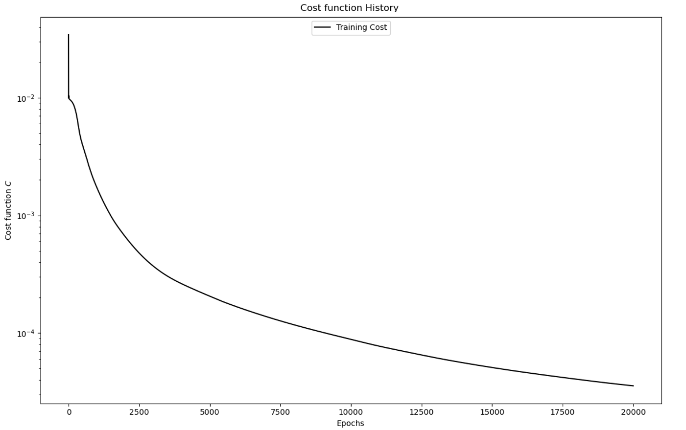
The best perfoming neural network was obtained using a combination of Linear and PReLu
PyTorch layers, reaching a cost of less than 5 x 10^-5 over 20,000 epochs. The training
history is shown in Figure 5. The evaluation of this model over the 676,00 points per file is done in 20 seconds.

Since the usage of the model is specific to vicinity of the laser, the melt pool profile
is used as a measure of the network’s performance. In Figure 6, the melt pool is observed
in two power and velocity levels where the non-absolute relative error of the prediction
is minimum and maximum.

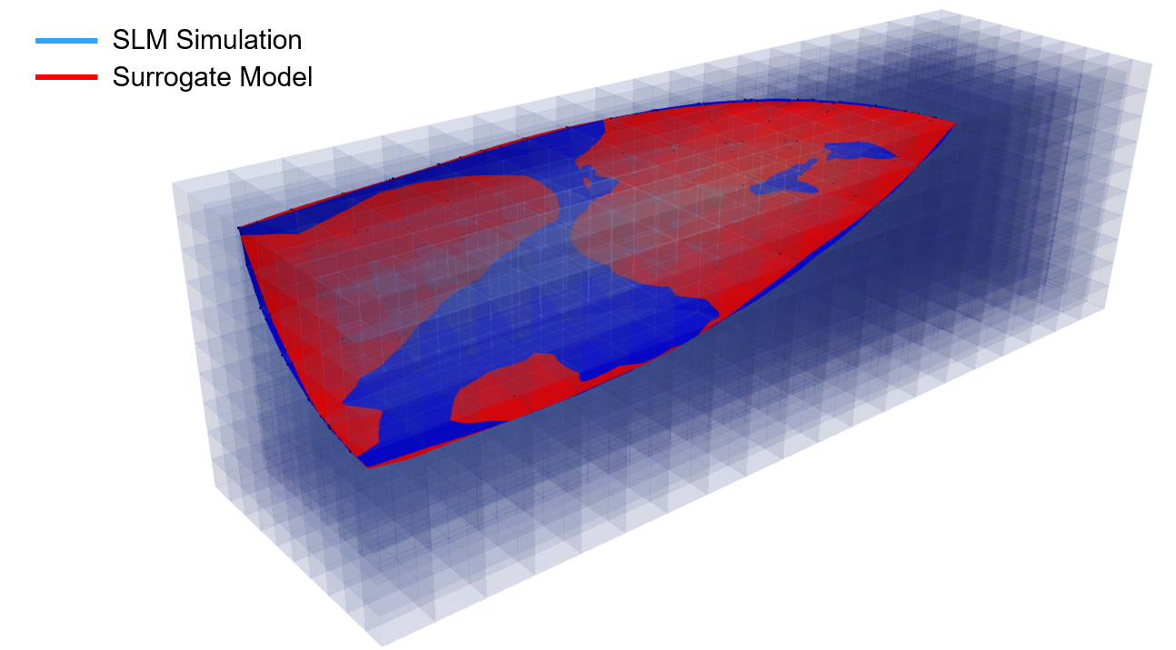
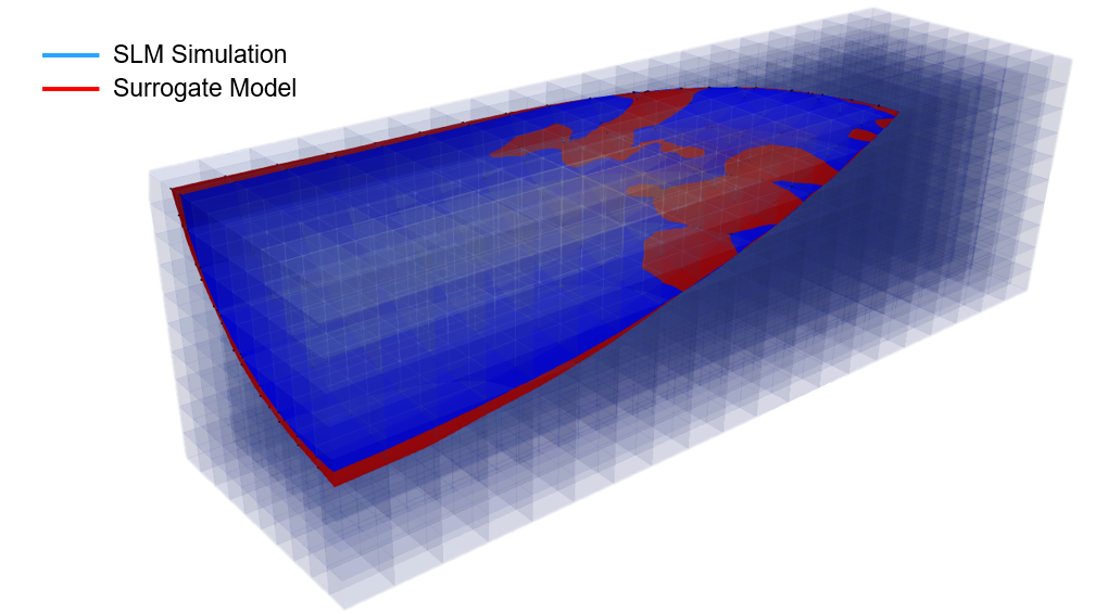
Despite of the slight differences, there is a large agreement between the overall shape
and size of the melt pool between the SLM simulation and the surrogate model. This agreement
is observed over the wide range of power levels and laser velocities.

Final Remarks and Outlook

Throughout this project, a modular workflow for training a neural network has been established where further
use was kept in mind while writing the code. This project has also offered a learning journey over the details
of training a neural network along with other aspects such as sampling, scaling, and layer types. Finally, a model
has been trained that offers accurate predictions of the melt pool within the span of seconds.

As for further steps in the short term, the performance of a model within the proposed usage of a multi-scale simulation is yet to
be evaluated, where the trade-off between speed and accuracy should be studied. Further, the model’s prediction would benefit from transfer learning, to further converge the melt pool
shape in the different ranges of power resulting as low, mid, and high-powered lasers. As for long term steps, convoluted neural networks
and physics informed neural networks are other options worth exploring within the project’s use case.

References