Martin Ruchti did his honours’ project at the Chair of Structural Analysis (TUM) and
was supervised by Michael André M.Sc., Máté Péntek M.Sc. and Dr.-Ing. Roland Wüchner
Introduction
More and more engineering tasks include not only an analysis of the performance of a system, but also a shape optimization. The general idea of shape optimization is, to modify a given setup in order to increase the performance with respect to a defined objective function I(D). Therefore, the design variables D are defined. In optimization, tree levels of detail are considered. Topology optimization modifies engineering systems on a coarse level, while sizing modifies the finest level of the system. Shape optimization is embedded in between topology optimization and sizing [2]. In this project, shape optimization is performed in the context of transient fluid simulation. The objective function I is defined as the drag force or as the lift force, an object in a flow exhibits. The design variables D are the nodal coordinates on the boundary.
Gradient based Optimization
While there is a great variety of optimization algorithms, using no gradient information, like evolutionary algorithms or genetic algorithms, those are in need of a relatively high number of objective function evaluations. Especially in transient flow problems, the objective function evaluations are computationally costly. Therefore, a gradient based approach is favorable. The most intuitive approach for numerical optimization is the steepest descend, described in [1]. In order to compute a gradient based shape optimization for the drag force and the lift force simultaneously, a modified step direction approach is introduced in Eq. 1.
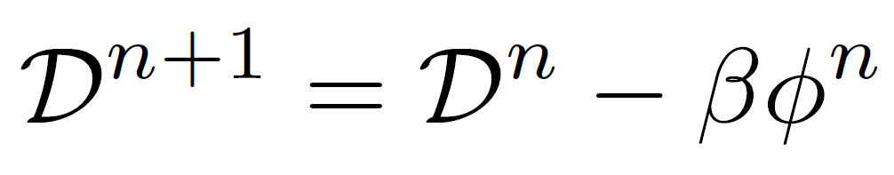 |
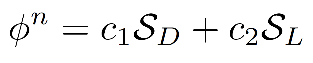
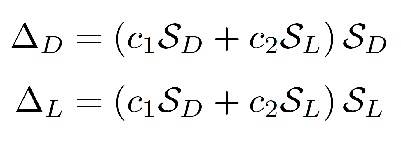
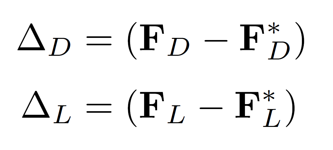
This step direction given in Eq. 2, is chosen, in order to satisfies the equation system Eq. 3. In this equation, SD denotes the drag force shape sensitivity and SL denotes the lift force shape sensitivity. The terms ΔD and ΔL are the deviation from the target values and are defined in Eq. 4. With the constants are computed by Eq. 5, the solution is estimated to converge to the given drag force target and lift force target in one step, with a step size β = 1.0. However, in order to stabilize the scheme, the step length is chosen as a number smaller than 1.0.
 |
 |
 |
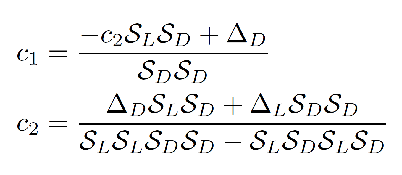 |
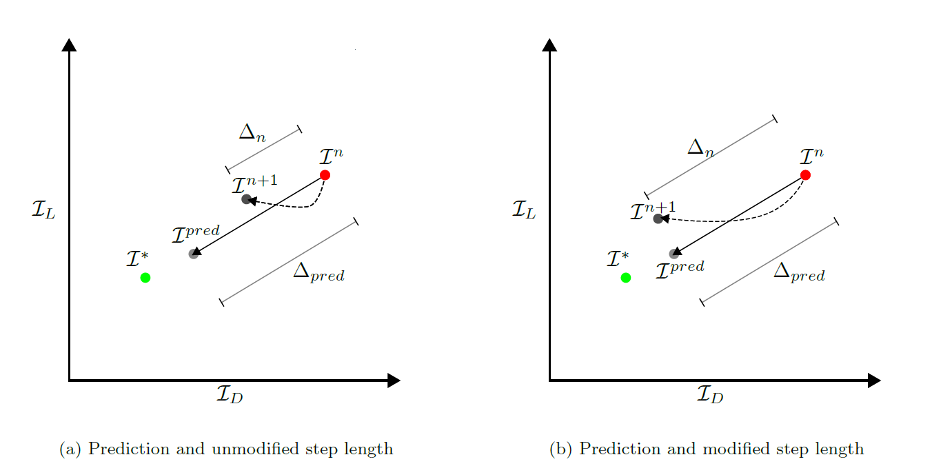
Since the response of the system in fluid dynamics is highly non-linear, the prediction is hardly exact. Therefore, the step length is modified in every optimization iteration by the equation Eq. 6. Therefore, the step length is adapted to the predicted step length. Figure Fig. 1 shows the effect of the modified step length.
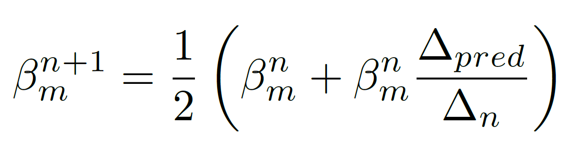 |
 |
Numerical Test Case
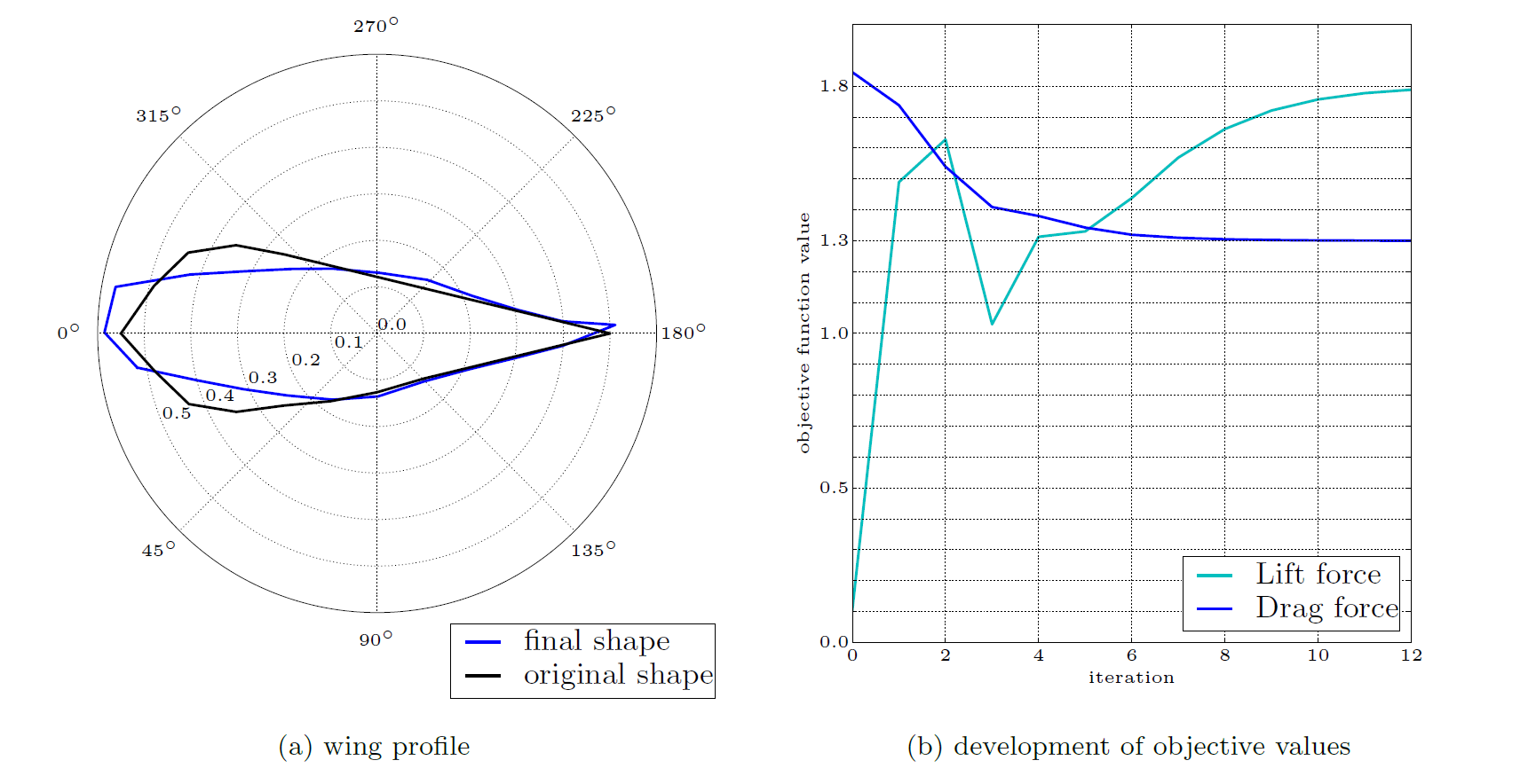
In order to test the scheme implemented in pyKratos [3] during this project, a wing profile in a flow is optimized. Therefore, an initially symmetric wing profile is placed in a flow with properties of air ν = 1.345e-5 [m2/s] and ρ = 1.0 [kg/m3]. The velocity v is chosen to be 1.0 [m/s]. The drag and lift forces are calculated for a time interval of 18.0 [s]. The lift force is optimized, to increase from initially 0.1 to 1.8, while the drag force is minimized from initially 1.83 to 1.3. The figure Fig. 2 shows the final shape of the wing profile, together with the objective function development. The optimization takes 12 steps to converge to the desired values. Figure Fig. 3 shows the change of the pressure distribution of the wing profile, during optimization. The result is visualized using GiD [4].
 |
 |
Result Accuracy
The result is defined as converged, if the drag force and lift force are within 1 % error to the target values 1.3 and 1.8. The wing profile optimization converged within 12 steps. The result accuracy was 0.68 %. Hence, the lift to drag ratio is increased from initially 0.0574, to 1.3756.
Conclusions
The shape optimization scheme proposed and implemented for this project, showed great success in optimizing drag force and lift force simultaneously. The result accuracy was found to be within the desired limits. For further improvement, an ALE mesh moving strategy could be included, to reduce limitations, inserted by the mesh. Since gradient based optimization is only exploitive and not explorative, a combined optimization method could be applied in order to search for promising prototype shapes, before the final result is obtained by a gradient based optimization.
References
| [1] | J. Nocedal and S. J. Wright Numerical Optimization Springer, Berlin, 2006 |
| [2] | K.-U. Bletzinger Structural Optimization Lecture notes, Technische Universität München, Winter 2014 |
| [3] | PyKratos, access: 2015-09-14 [ http ] |
| [4] | GiD, access: 2015-09-14 [ http ] |