Supervision: Philipp Neumann, Alexander Breuer, and Kristof Unterweger
Project Description
During the project the team of students worked on coupling two frameworks for numerical simulation. First, Clawpack includes various solvers for hyperbolic equations implemented in Fortran. Clawpack stands for “Conservation Laws Package” and was initially developed for linear and nonlinear hyperbolic systems of conservation laws, with a focus on implementing high-resolution Godunov type methods using limiters in a general framework applicable to many applications. PyClaw was designed as a Python wrapper for Clawpack in order to simplify the set-up of the numerical experiment. Another framework – Peano – was created for traversing adaptive Cartesian grids with automatic traversal. The idea of this project was to exploit scripting advantages of Python and to use a third-party solver on a Peano grid. The main focus of the project was in porting the existing 2D code to also work in three dimensions. To solve the acoustic equations numerically, the theory of the hyperbolic wave equations was investigated. A Finite Volume method with dimensional splitting was used as the numerical method. PyClaw contains a set of algorithms and methods for solving such hyperbolic equations.
3D PeanoClaw
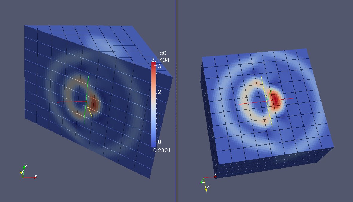
Figure 1: Cross section through a three-dimensional domain.
Finally, a working three-dimensional application was obtained, solving the acoustics equation (Fig. 1). To exploit the featuers of the coupled approach, different scenarios with adaptive grids and complex media properties were successfully tested (Fig. 2).
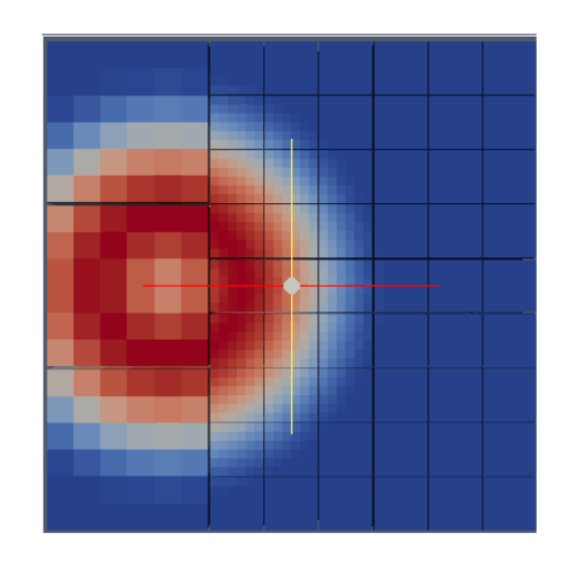
Figure 2: Spherical wave in a refined grid. Left and right parts of the domain have different acoustic impedances.
Validation
In order to validate the results of 3D PeanoClaw with multiple patches, its results are compared against the results obtained by PyClaw for the same scenario. The comparison of results is visualised in Fig 3. As it is shown in this figure the observed differences are close to machine precision.
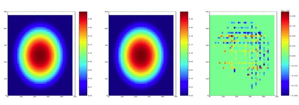
Figure 3: 3D spherical wave computed in PeanoClaw (left) and PyClaw (middle), and the resulting error (right).