Julia Fischer did her honours’ project at the at the Institute for Computational Mechanics (TUM).
She was supervised by Svenja Schoeder M.Sc. and Prof. Dr.-Ing. Wolfgang A. Wall.
Introduction
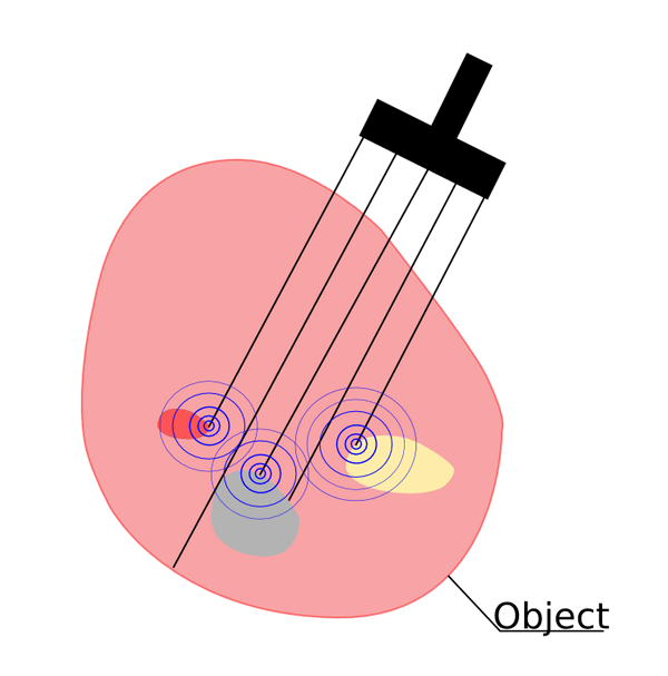
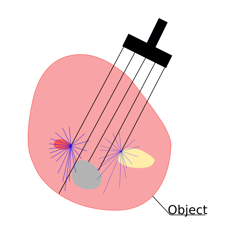
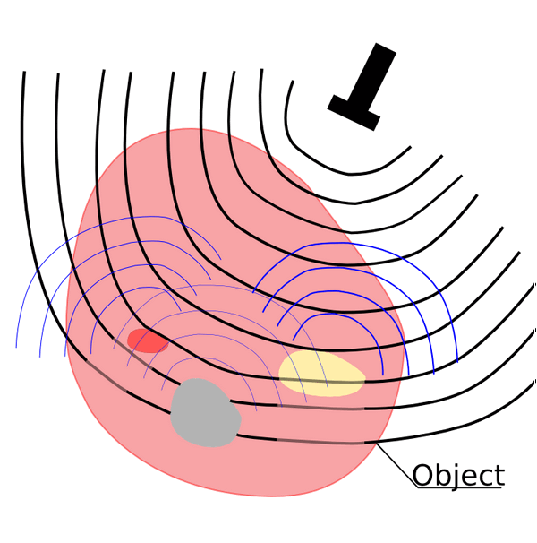
Photoacoustic tomography (PAT) offers a new field of research as medical imaging method. It is used to achieve optical contrast and high acoustical resolution at the same time. An object of interest is illuminated by a laser pulse (see Fig. 1.a). At the impact, optical energy is absorbed and transferred to heat. The rapid rise in temperature leads to emission of pressure waves due to thermal expansion. The pressure waves are then detected by acoustical transducers located at the boundary [1]. Reconstruction algorithms are used to form the recorded data sets to high quality images [2]. Photoacoustic tomography can be thought as combination of diffuse optical tomography (see Fig. 1.b) and ultrasonography (see Fig. 1.c) via the photoacoustic effect.
 |
 |
 |
|
(a) Photoacoustic tomography
|
(b) Diffuse optical tomography
|
(c) Ultrasonography
|
Computational Remarks
To solve the coupled problem, the light problem is discretized using the standard finite element method. The hybridizable discontinuous Galerkin method is used for the acoustic problem. For the time discretization, Euler, backward differentiation (BDF) or diagonal implicit Runge-Kutta (DIRK) schemes are applied. All quantities – the absorption coefficient μa, the diffusion coefficient D, the optical flux Φ and the initial pressure p0 – are discrete and defined on element level. The initial pressure for the sound propagation is calculated in dependency of the solution Φ of the optical problem. For this, a mapping is carried out.
Reconstruction of the scattering distribution
In order to reconstruct the scattering distribution within tissues, an optimization with respect to the diffusion coefficient D is performed. For this, the objective function J is minimized. The objective J describes the difference between measured and simulated pressure values at the monitored boundary. Minimizing the objective w.r.t. D, i.e. calculating the gradient of the objective function is equivalent to the partial derivative of the Lagrange function L.
Regularization
Extending the objective function by an additional term, a stabilized solution of an ill-posed problem can be found [4] and noise can be removed. For this, Tikhonov or total variation diminishing (TVD) regularization can be used. α is the regularization parameter which can be modified in order to improve convergence.
Examples
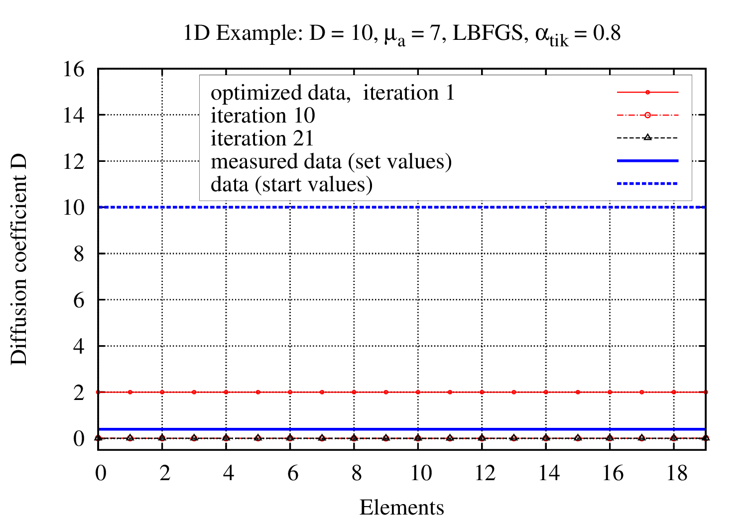
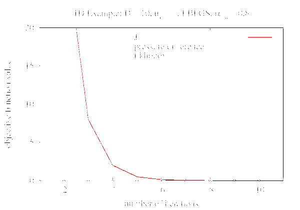
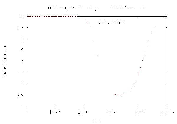
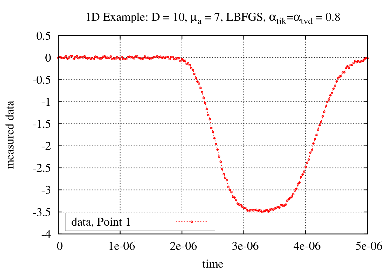
The figure 2.a shows a simple 1D example. Forward data is generated with constant μa = 7 and D = 0.4. This corresponds to the properties of muscles. An inverse analysis is performed with start values μa = 7 and D= 10. The development of the scattering coefficient is shown. The simulation is able to reconstruct the forward data. Figure 2.b shows the development of the objective function value. Pressure is measured at the monitored boundary. Figure 3.a shows the initial pressure distribution. In order to study the effect of noise, the pressure distribution of figure 3.a is modified. Figure 3.b shows the pressure distribution of figure 3.a including 1% noise.
 |
 |
|
(a) Development of Diffusion coefficient D
|
(b) Development of objective function value
|
 |
 |
|
(a) Initial pressure distribution
|
(b) Modified pressure distribution with 1% artificial noise
|
Conclusion
Using gradient based optimization, the distribution of the scattering coefficient can be reconstructed. However, additional artificial noise in forward data delivers insufficient results. Optimization w.r.t. to both optical parameters at the same time only results in good approximations for the absorption coefficient due to non-uniqueness and ill conditioning. The quality of the approximations for the Diffusion coefficient strongly depends on the geometry and the right choice of the regularization parameter α. Therefore, a sensitivity analysis needs to be performed.