Leon Herrmann did his honours project at the Chair of Computational Modeling and Simulation (TUM) and was supervised by PD Dr.-Ing. habil. Stefan Kollmannsberger and Davide D’Angella, M.Sc. (hons)
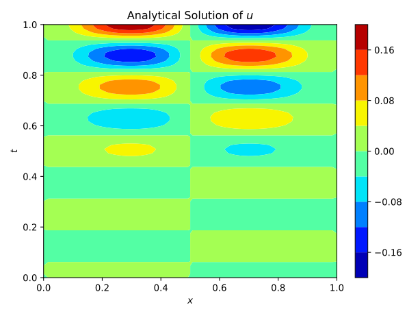
The acoustic wave equation describes the wave propagation through a material. Its solution is a pressure field u(x,t) depending both on the spatial and temporal domain. An example of a solution of a 1D case is shown in figure 1. The waves are initiated by initial conditions, boundary conditions or an external source. The speed, at which the acoustic waves travel is governed by the wave speed vp(x), which is a material property related to the elastic modulus and the mass density. This property may vary throughout the material and indicate a flaw if it is significantly lower than in the remaining specimen. This fact can be used for non-destructive testing, where the pressure induced by an ultrasonic signal is measured at the boundary of the material and then used to infer the distribution of the wave-velocity. This is an inverse problem and ill-posed. There is no guarantee for a unique solution. Inverse problems pose difficulties for conventional approaches. One method of solving the inverse problem is the Full-Waveform inversion [1], [2].
 |
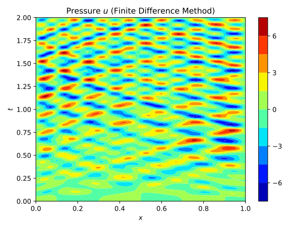 |
Fig.1: Example solution of a 1D wave equation. The crosses at x=0.1, x=0.9 indicate possible measurements of the pressure.
Another interesting option for solving the inverse problem is by using Deep Learning. The field experienced rapid growth in recent years and it is therefore of interest to also apply the discoveries in Deep Learning to Physics and Engineering. This has already been done and especially the application for inverse problems seems promising, as these have not yet been solved satisfactorily with conventional approaches.
For this task, Artificial Neural Networks will be used. These can be regarded as universal function approximators [3]. The Neural Networks are composed of learnable weights and biases. Given an input x, the network predicts an output y. The output y can then be used to compute a cost function, which quantifies the quality of the output y. Through automatic differentiation [4], the gradients of the cost function w.r.t. the weights and biases can be computed. The gradients are then used together with a gradient descent algorithm [4] to adjust the weights and biases, such that the cost function is minimized. This is how Neural Networks are trained.
Several learning approaches are investigated. These can be classified into two categories, Forward Solvers and Inverse Solvers:
- Forward Solvers
- Physics Informed Neural Networks
- Physics Informed Neural Networks for surrogate modeling
- Learning a time-stepping scheme
- Inverse Solvers
- Iterative Solver
- Physics Informed Inverse Solver
- Data-driven Inverse Solver
- Deep-Learning Inversion
Physics Informed Neural Networks [5] use a neural network to predict the solution of a differential equation y(x) from the coordinates x. The cost function is then defined by the residual of the corresponding differential equation, which is minimized to learn the correct solution y(x). This training process is very expensive compared to conventional approaches, such as finite elements or finite differences. As the wave equation can be solved efficiently with e.g. finite differences, this approach does not seem very useful.
However, Physics Informed Neural Networks have been extended for surrogate modeling by [6]. The idea is to extend the network with additional input information. For the wave equation, the network would then predict the pressure u(x,t) from the coordinates x, time t and the wave velocity vp(x). Additionally Convolutional Neural Networks (CNN) [4] are used instead of Fully-Connected Neural Networks (FC-NN). The advantage of these is that they are shift-invariant, which makes them good for image analysis. The wave velocity distribution and the pressure field and can be interpreted as 1D and 2D images. This is why it makes sense to introduce CNNs to the network architecture. The specific architecture, that was used is a Densely connected convolutional network [7].
To test the approach it was first applied to a single wave velocity distribution, so without surrogate modeling capabilities. The neural network, consisting of 33’754 parameters and 15 convolutional layers, predicts the entire pressure field from a single wave-velocity distribution. The results are illustrated in figure 2. It is seen, that it achieves an acceptable accuracy.
 |
 |
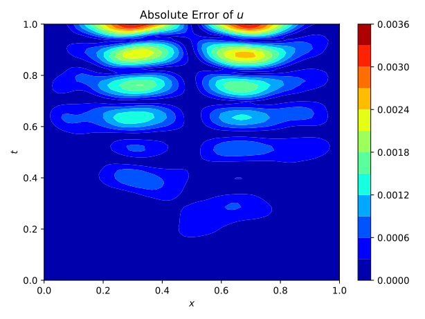 |
Fig.2: Prediction and Solution of the wave equation using Physics Informed Neural Networks.
The training time is about 450 s. This can be compared to the original Physics Informed Neural Networks, which took about 1000 s. Although it is an improvement, it is still too expensive compared to a finite difference scheme, which takes about 0.04 s. However, if the network can be trained to work with multiple wave velocities, it is viable to accept a high training time, if the prediction time is low. The prediction time for this network is 0.002 s, so a significant improvement to the finite difference scheme. This difference becomes even more significant with a finer grid and higher dimensionality. It is therefore of interest to investigate this approach further. It has to however be noted, that the minimization process is very difficult and highly dependant on the network architecture. This is the reason, why no successful implementation could be provided in the context of this project.
An alternative approach presented by [8] is the Learning of a time-stepping scheme. The idea is to use a network to predict the next time step given a specific number of previous time steps. The training occurs via a comparison of the prediction to values obtained by a conventional time-stepping scheme. The goal is to create a Neural Network, that can compute larger and cheaper timesteps. As an architecture, it also uses a Densely connected convolutional network. Although this approach seems great for dynamic problems, the given task of solving the inverse wave equation poses several complications. First, the additional source term has to be taken into account in the network. Then different wave velocity distributions have to be provided, to create a useful surrogate model. Finally, it is not even guaranteed, that larger timesteps will help to resolve the inverse problem. This approach was therefore not investigated further.
Several approaches, that are used for the inverse problem require a forward solver. In the following, this will be done with finite differences. It has however been shown, that there is a potential for improvement by using a trained Physics Informed Neural Network as a surrogate model.
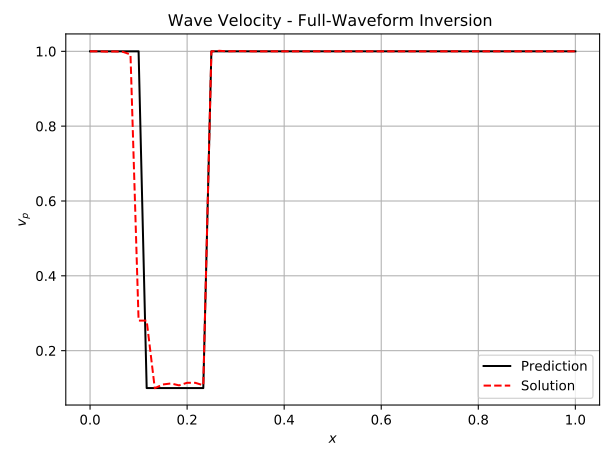
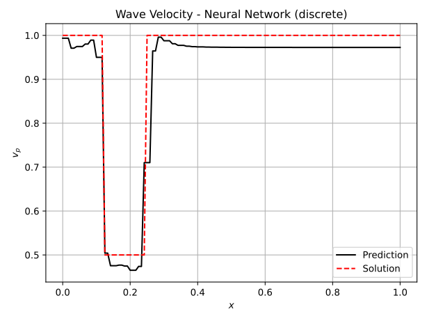
The iterative approach is inspired by the Full-Waveform inversion [1], [2], where a misfit functional is minimized iteratively by solving the forward and adjoint problem. Here it has been adjusted for Neural Networks. The Neural Network predicts the wave velocity vp(x) from the coordinates x. The predicted wave velocity is then used to compute the pressure field using the finite difference method. The pressure field is then compared to a prior measurement of the true pressure field. The difference is used as the cost function and minimized so that a better prediction of the wave velocity is achieved. To simplify the learning process, shape functions can be used to approximate the wave velocity. In this case, the Neural Network predicts the coefficients of the shape functions. This approach is called the discrete method, whereas the previous approach is denoted as continuous. The results are shown in figure 3, where a comparison is also made to the Full-Waveform inversion. Note, that the measurements were taken along the entire spatio-temporal domain.
 |
 |
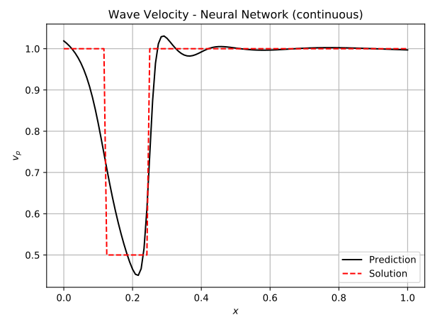 |
Fig.3: Predictions of the wave velocity using Full-Waveform Inversion, the discrete Inverse Solver and the continuous Inverse Solver. Note, that measurements of the pressure have been taken along the entire domain.
For non-destructive testing, it is usually not possible to measure along the entire domain. Therefore the approaches have also been tested with measurements at only x=0.1 and x=0.9. The iterative method using Neural Networks still predicts the flaw very well. For the continuous version, this is shown in figure 4. A FC-NN with three hidden layers and 100 Neurons was used for this task. The training takes about 250 s, which is significantly greater than for the Full-Waveform inversion, which takes 30 s.
 |
 |
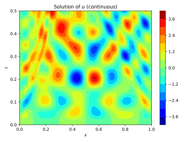 |
Fig.4: The learning process of the continuous Inverse Solver for 1000 epochs. The pressure measurements are indicated in the center figure with the white lines at x=0.1, x=0.9.
An alternative is to use both a Neural Network for the task of predicting the pressure field and the wave velocity. This is denoted as the Physics Informed Inverse Solver and inspired by [5], [9], [10]. The wave velocity is predicted from the coordinates and the pressure field u from both the coordinates and time. The cost function is then defined by both the residual of the differential equation and the error between the prediction and measurement of the pressure field. The training of the networks occurs sequentially, which is illustrated in figure 5, where first the pressure field u(x,t) is learned and subsequently the wave velocity distribution vp(x). It has to be remarked, that this only worked for pressure measurements along the entire spatio-temporal domain. Training times were around 300 s. Due to the requirement of data throughout the entire domain, the approach does not seem very promising. Similar approaches have however been shown to be very successful for more complex inverse problems, where the underlying form of the differential equation is unknown [9], [10].
 |
 |
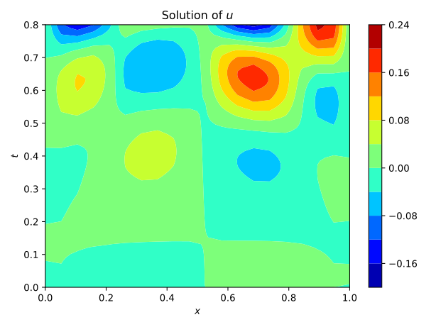 |
Fig.5: The learning process of the Physics Informed Inverse Solver for 1000 epochs. The pressure measurements have been taken along the entire domain. Note, that learning occurs sequentially. During the first 500 epochs the pressure is learned and during the last 500 epochs the wave velocity.
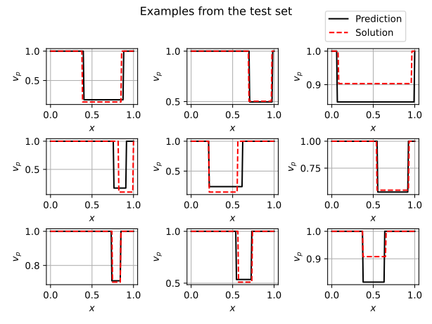
Lastly, a data-driven approach was investigated. The data-driven Inverse Solver relies solely on data and does not take the physics into account anymore. The approach was inspired by [10], where parametrized flaws were detected in 2D domains. The idea is to parametrize the wave velocity with a step function. It is assumed, that the unflawed material has a wave velocity vp(x)=1. The flaw can then be described by three parameters, the flaw length, depth, and position. A Neural Network is then used to predict the three parameters from two measurements of the pressure field at x=0.1 and x=0.9. A labeled training dataset of 2500 cases is then generated with the finite difference method. The cost function is defined by the difference between the predicted parameters and the label. The chosen network is a combination of a CNN and a FC-NN. Predictions from a different testing dataset are shown in figure 5. It is seen, that the predictions are quite reliable. Training of the network takes about 90 s and the prediction of the entire testing dataset composed of 2500 cases takes 0.0005 s. Therefore a data-driven approach also seems very promising. It has to however be noted, that the creation of the datasets might be very expensive and thereby not necessarily viable.
 |
Alternatively, it is proposed by [12] to directly predict the wave velocity from the measurements by using a fully convolutional network [13]. The approach is called Deep-Learning Inversion and very similar to the previously described approach. The only difference is, that the wave velocity is no longer parametrized and more general predictions can be made. The approach has not been investigated, but due to the described successes in [12] and the success with the data-driven inverse solver, an implementation for the 1D wave equation for comparison seems beneficial.